(This post was last updated on 2022-12-31.)
In this blog, I explore whether the extent of shrinkage depends on the number of trials. To do so, I simulate three data sets with different trial numbers for each participant and then visualize the shrinkage.
1 Setup
# load the libraries
library(tidyverse)
library(faux)
library(lme4)
The general population parameters used to simulate the three data sets are as following:
# population parameters
N_subj <- 40

# fixed effects
fix_int <- 4
fix_slp <- 2

# random effects
sd_int <- 1 # sd of the random intercept
sd_slp <- 1 # sd of the random slope
cor_subj <- 0.5 # correlation between random effects

sgm <- 1 # sigma
In a nutshell, the hypothetical experiment incorporates one independent variable (IV) with two levels (a1 vs a2), where data for 40 participants are simulated.
2 With the same number of trials (80)
In the first simulated data, there are 80 trials in each condition for each participant.
2.1 Simulating data
Simulate the data set:
set.seed(2022)

df_sameL_full <-
  add_random(subj=N_subj) %>%
  add_random(trial=80) %>% # 80 trials per participant
  add_within(IV = c("a1", "a2")) %>%
  add_contrast("IV", "treatment", colnames = "IV_code") %>%
  add_ranef("subj", rand_int = sd_int, rand_slp = sd_slp, .cors=cor_subj) %>%
  add_ranef(sigma = sgm) %>%
  mutate(DV = (fix_int + rand_int) +          # intercept
           (fix_slp + rand_slp) * IV_code +   # slope
           sigma)                             # sigma

df_sameL <- df_sameL_full %>%
  select(Subj=subj, IV, IV_code, Trial=trial, DV)

str(df_sameL)
## tibble [6,400 × 5] (S3: tbl_df/tbl/data.frame)
## $ Subj : chr [1:6400] "s01" "s01" "s01" "s01" ...
## $ IV : Factor w/ 2 levels "a1","a2": 1 2 1 2 1 2 1 2 1 2 ...
## ..- attr(*, "contrasts")= num [1:2, 1] 0 1
## .. ..- attr(*, "dimnames")=List of 2
## .. .. ..$ : chr [1:2] "a1" "a2"
## .. .. ..$ : chr ".a2-a1"
## $ IV_code: num [1:6400] 0 1 0 1 0 1 0 1 0 1 ...
## $ Trial : chr [1:6400] "t01" "t01" "t02" "t02" ...
## $ DV : num [1:6400] 3.9 9.43 5.99 6.48 2.72 ...The numbers of trials in each condition are:
df_sameL %>%
  group_by(Subj, IV) %>%
  summarize(N = n(), .groups = "drop") %>%
  pivot_wider(names_from = IV, values_from = N)
2.2 Individual estimates
We first estimate the intercepts and slopes for each participant separately (as researchers usually do when employing ANOVAs):
eff_sameL <- df_sameL %>%
  group_by(Subj, IV) %>%
  summarize(avgDV = mean(DV), .groups = "drop") %>%
  pivot_wider(names_from = IV, values_from = avgDV) %>%
  transmute(Subj,
            indi_int = a1,
            indi_slp = a2-a1)

head(eff_sameL)
2.3 LMM-fitted means
Then we estimate the intercepts and slopes for each participant with linear mixed-effects models:
lmm_sameL <- lmer(DV ~ IV + (IV | Subj),
                  data = df_sameL)
summary(lmm_sameL)
## Linear mixed model fit by REML ['lmerMod']
## Formula: DV ~ IV + (IV | Subj)
## Data: df_sameL
##
## REML criterion at convergence: 18359
##
## Scaled residuals:
## Min 1Q Median 3Q Max
## -3.486 -0.681 -0.001 0.673 3.749
##
## Random effects:
## Groups Name Variance Std.Dev. Corr
## Subj (Intercept) 0.751 0.867
## IV.a2-a1 0.842 0.917 0.48
## Residual 0.980 0.990
## Number of obs: 6400, groups: Subj, 40
##
## Fixed effects:
## Estimate Std. Error t value
## (Intercept) 3.837 0.138 27.8
## IV.a2-a1 2.020 0.147 13.7
##
## Correlation of Fixed Effects:
## (Intr)
## IV.a2-a1 0.453Extract the intercepts and slopes for each participant:
eff_sameL <- ranef(lmm_sameL) %>%
  as.data.frame() %>%
  transmute(Subj = grp,
            effect = if_else(term=="(Intercept)", "lmm_int", "lmm_slp"),
            condval) %>%
  pivot_wider(names_from = effect, values_from = condval) %>%
  mutate(lmm_int = lmm_int + fixef(lmm_sameL)[1],
         lmm_slp = lmm_slp + fixef(lmm_sameL)[2]) %>%
  inner_join(eff_sameL, by="Subj")

eff_sameL
2.4 Shrinkage
Put all estimates in one data frame:
eff_sameL_long <- eff_sameL %>%
  pivot_longer(contains("_"), names_to = c("Method", "effect"), names_sep="_") %>%
  mutate(effect = if_else(effect=="int", "intercept", "slope"),
         Method = as_factor(Method),
         Method = fct_rev(Method))

str(eff_sameL_long)
## tibble [160 × 4] (S3: tbl_df/tbl/data.frame)
## $ Subj : chr [1:160] "s01" "s01" "s01" "s01" ...
## $ Method: Factor w/ 2 levels "indi","lmm": 2 2 1 1 2 2 1 1 2 2 ...
## $ effect: chr [1:160] "intercept" "slope" "intercept" "slope" ...
## $ value : num [1:160] 4.73 2.84 4.73 2.85 2.61 ...Visualize the shrinkage:
plot_sameL <- eff_sameL_long %>%
  pivot_wider(names_from = effect, values_from = value) %>%
  mutate(rowname = if_else(Method=="lmm", Subj, ""),
         Method = fct_recode(Method,
                             `LMM-fitted`="lmm",
                             Individual="indi")) %>%
  ggplot(aes(intercept, slope)) +
  geom_point(aes(color=Method)) +
  scale_color_manual(values=c("blue", "red")) +
  coord_cartesian(x=c(1.7, 5.4), y=c(-.85, 3.65)) +
  geom_line(aes(group=Subj), linetype="dashed") +
  geom_point(aes(x = fixef(lmm_sameL)[1],
                 y = fixef(lmm_sameL)[2]),
             size = 7, colour = 'red', alpha = 0.05) +
  geom_point(aes(
    x = mean(eff_sameL$indi_int),
    y = mean(eff_sameL$indi_slp)),
    size = 4, colour = 'blue', alpha = 0.05) +
  theme(legend.title = element_blank())

plot_sameL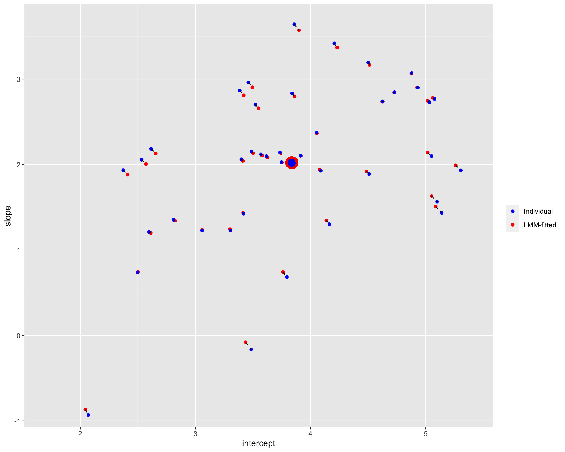
Note: The blue points denote the individual estimates while the red points denote the estimates from linear mixed-effects models. The dashed line connects different estimates for the same participant; the distance between estimates could be understood as the extent of shrinkage. The large points are the population estimates (across all participants).
It seems that the extend of shrinkage is (relatively) small when the trial numbers are large.
3 With the same number of trials (20)
In the second simulated data, there are 20 trials in each condition for each participant.
3.1 Simulating data
Simulate the data set:
set.seed(2022)

df_sameS_full <-
  add_random(subj=N_subj) %>%
  add_random(trial=10) %>% # 50 trials per participant
  add_within(IV = c("a1", "a2")) %>%
  add_contrast("IV", "treatment", colnames = "IV_code") %>%
  add_ranef("subj", rand_int = sd_int, rand_slp = sd_slp, .cors=cor_subj) %>%
  add_ranef(sigma = sgm) %>%
  mutate(DV = (fix_int + rand_int) +          # intercept
           (fix_slp + rand_slp) * IV_code +   # slope
           sigma)                             # sigma

df_sameS <- df_sameS_full %>%
  select(Subj=subj, IV, IV_code, Trial=trial, DV)

str(df_sameS)
## tibble [800 × 5] (S3: tbl_df/tbl/data.frame)
## $ Subj : chr [1:800] "s01" "s01" "s01" "s01" ...
## $ IV : Factor w/ 2 levels "a1","a2": 1 2 1 2 1 2 1 2 1 2 ...
## ..- attr(*, "contrasts")= num [1:2, 1] 0 1
## .. ..- attr(*, "dimnames")=List of 2
## .. .. ..$ : chr [1:2] "a1" "a2"
## .. .. ..$ : chr ".a2-a1"
## $ IV_code: num [1:800] 0 1 0 1 0 1 0 1 0 1 ...
## $ Trial : chr [1:800] "t01" "t01" "t02" "t02" ...
## $ DV : num [1:800] 3.9 9.43 5.99 6.48 2.72 ...The numbers of trials in each condition are:
df_sameS %>%
  group_by(Subj, IV) %>%
  summarize(N = n(), .groups = "drop") %>%
  pivot_wider(names_from = IV, values_from = N)
3.2 Individual estimates
We first estimate the intercepts and slopes for each participant separately (as researchers usually do when employing ANOVAs):
eff_sameS <- df_sameS %>%
  group_by(Subj, IV) %>%
  summarize(avgDV = mean(DV), .groups = "drop") %>%
  pivot_wider(names_from = IV, values_from = avgDV) %>%
  transmute(Subj,
            indi_int = a1,
            indi_slp = a2-a1)

head(eff_sameS)
3.3 LMM-fitted means
Then we estimate the intercepts and slopes for each participant with linear mixed-effects models:
lmm_sameS <- lmer(DV ~ IV + (IV | Subj),
                  data = df_sameS)
summary(lmm_sameS)
## Linear mixed model fit by REML ['lmerMod']
## Formula: DV ~ IV + (IV | Subj)
## Data: df_sameS
##
## REML criterion at convergence: 2424
##
## Scaled residuals:
## Min 1Q Median 3Q Max
## -2.9179 -0.6912 -0.0027 0.6470 3.0290
##
## Random effects:
## Groups Name Variance Std.Dev. Corr
## Subj (Intercept) 0.762 0.873
## IV.a2-a1 0.882 0.939 0.46
## Residual 0.965 0.982
## Number of obs: 800, groups: Subj, 40
##
## Fixed effects:
## Estimate Std. Error t value
## (Intercept) 3.773 0.146 25.8
## IV.a2-a1 2.098 0.164 12.8
##
## Correlation of Fixed Effects:
## (Intr)
## IV.a2-a1 0.288Extract the intercepts and slopes for each participant:
eff_sameS <- ranef(lmm_sameS) %>%
  as.data.frame() %>%
  transmute(Subj = grp,
            effect = if_else(term=="(Intercept)", "lmm_int", "lmm_slp"),
            condval) %>%
  pivot_wider(names_from = effect, values_from = condval) %>%
  mutate(lmm_int = lmm_int + fixef(lmm_sameS)[1],
         lmm_slp = lmm_slp + fixef(lmm_sameS)[2]) %>%
  inner_join(eff_sameS, by="Subj")

eff_sameS
3.4 Shrinkage
Put all estimates in one data frame:
eff_sameS_long <- eff_sameS %>%
  pivot_longer(contains("_"), names_to = c("Method", "effect"), names_sep="_") %>%
  mutate(effect = if_else(effect=="int", "intercept", "slope"),
         Method = as_factor(Method),
         Method = fct_rev(Method))

str(eff_sameS_long)
## tibble [160 × 4] (S3: tbl_df/tbl/data.frame)
## $ Subj : chr [1:160] "s01" "s01" "s01" "s01" ...
## $ Method: Factor w/ 2 levels "indi","lmm": 2 2 1 1 2 2 1 1 2 2 ...
## $ effect: chr [1:160] "intercept" "slope" "intercept" "slope" ...
## $ value : num [1:160] 5.16 2.72 5.35 2.52 2.7 ...Visualize the shrinkage:
plot_sameS <- eff_sameS_long %>%
  pivot_wider(names_from = effect, values_from = value) %>%
  mutate(rowname = if_else(Method=="lmm", Subj, ""),
         Method = fct_recode(Method,
                             `LMM-fitted`="lmm",
                             Individual="indi")) %>%
  ggplot(aes(intercept, slope)) +
  geom_point(aes(color=Method)) +
  coord_cartesian(x=c(1.7, 5.4), y=c(-.85, 3.65)) +
  scale_color_manual(values=c("blue", "red")) +
  geom_line(aes(group=Subj), linetype="dashed") +
  geom_point(aes(x = fixef(lmm_sameS)[1],
                 y = fixef(lmm_sameS)[2]),
             size = 7, colour = 'red', alpha = 0.05) +
  geom_point(aes(
    x = mean(eff_sameS$indi_int),
    y = mean(eff_sameS$indi_slp)),
    size = 4, colour = 'blue', alpha = 0.05)

plot_sameS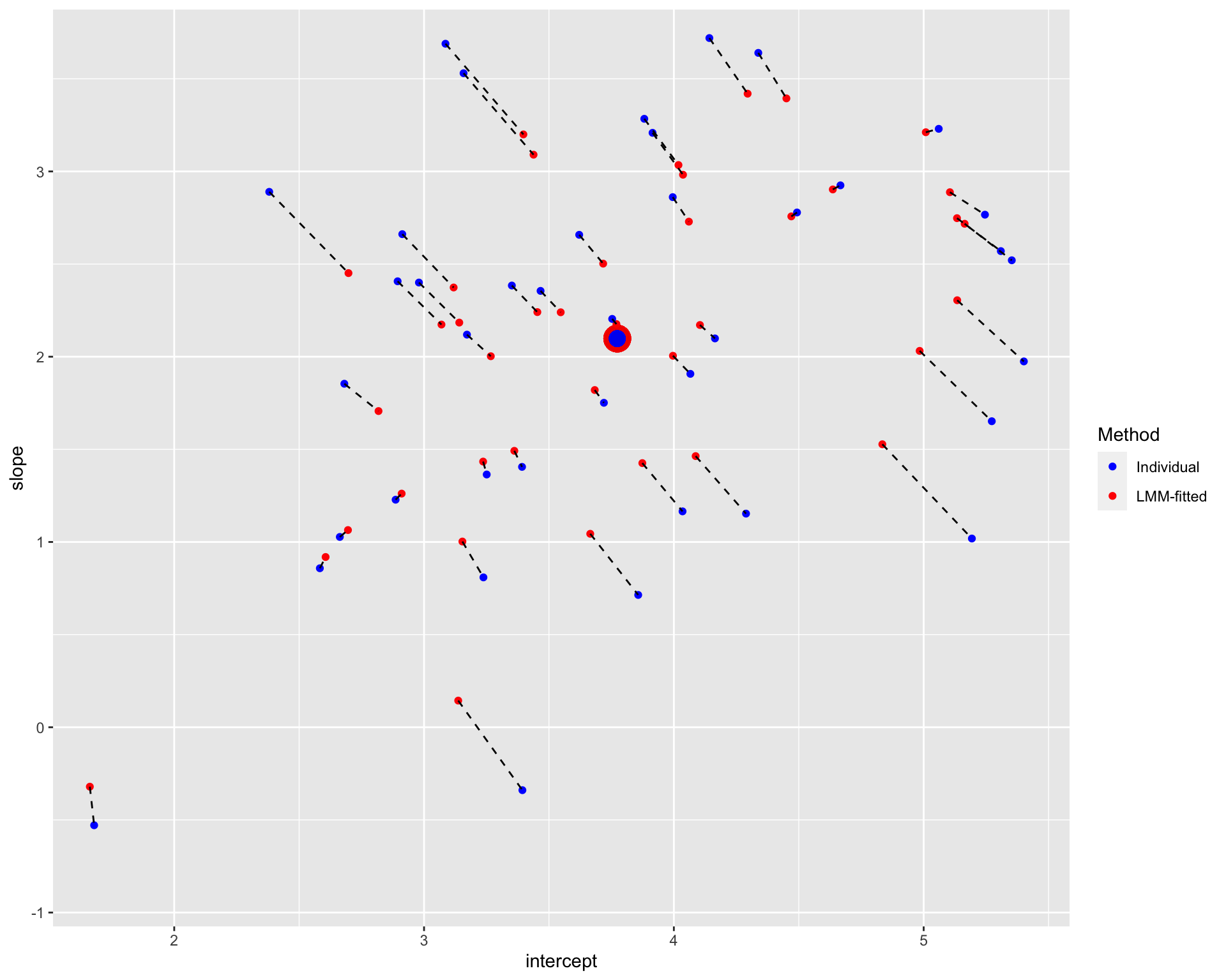
Note: The blue points denote the individual estimates while the red points denote the estimates from linear mixed-effects models. The dashed line connects different estimates for the same participant; the distance between estimates could be understood as the extent of shrinkage. The large points are the population estimates (across all participants).
It seems that the extend of shrinkage is (relatively) large when the trial numbers are small, especially for participants who are further away from the population estimates.
4 Contrast the shrinkage in the first two data sets
Combine and visualize the estimates:
bind_rows(eff_sameL_long %>%
            pivot_wider(names_from = effect, values_from = value) %>%
            mutate(rowname = if_else(Method=="lmm", Subj, ""),
                   Method = fct_recode(Method,
                                       `LMM-fitted`="lmm",
                                       Individual="indi"),
                   N = 80,
                   Subj_N = paste(Subj, N, sep="_"),
                   Subj_LMM = if_else(Method=="LMM-fitted", Subj,
                                      paste0(Subj, 1))),
          eff_sameS_long %>%
            pivot_wider(names_from = effect, values_from = value) %>%
            mutate(rowname = if_else(Method=="lmm", Subj, ""),
                   Method = fct_recode(Method,
                                       `LMM-fitted`="lmm",
                                       Individual="indi"),
                   N = 20,
                   Subj_N = paste(Subj, N, sep="_"),
                   Subj_LMM = if_else(Method=="LMM-fitted", Subj,
                                      paste0(Subj, 2)))) %>%
  mutate(`Trial No.` = factor(N)) %>%
  ggplot(aes(intercept, slope)) +
  geom_point(aes(color=Method, shape=`Trial No.`)) +
  coord_cartesian(x=c(1.7, 5.4), y=c(-.85, 3.65)) +
  scale_color_manual(values=c("blue", "red")) +
  geom_line(aes(group=Subj_N), linetype="dashed") +
  geom_line(aes(group=Subj_LMM), linetype="dotted") +
  geom_point(aes(x = fixef(lmm_sameS)[1],
                 y = fixef(lmm_sameS)[2]),
             size = 7, colour = 'red', alpha = 0.05) +
  geom_point(aes(
    x = mean(eff_sameS$indi_int),
    y = mean(eff_sameS$indi_slp)),
size = 4, colour = 'blue', alpha = 0.05)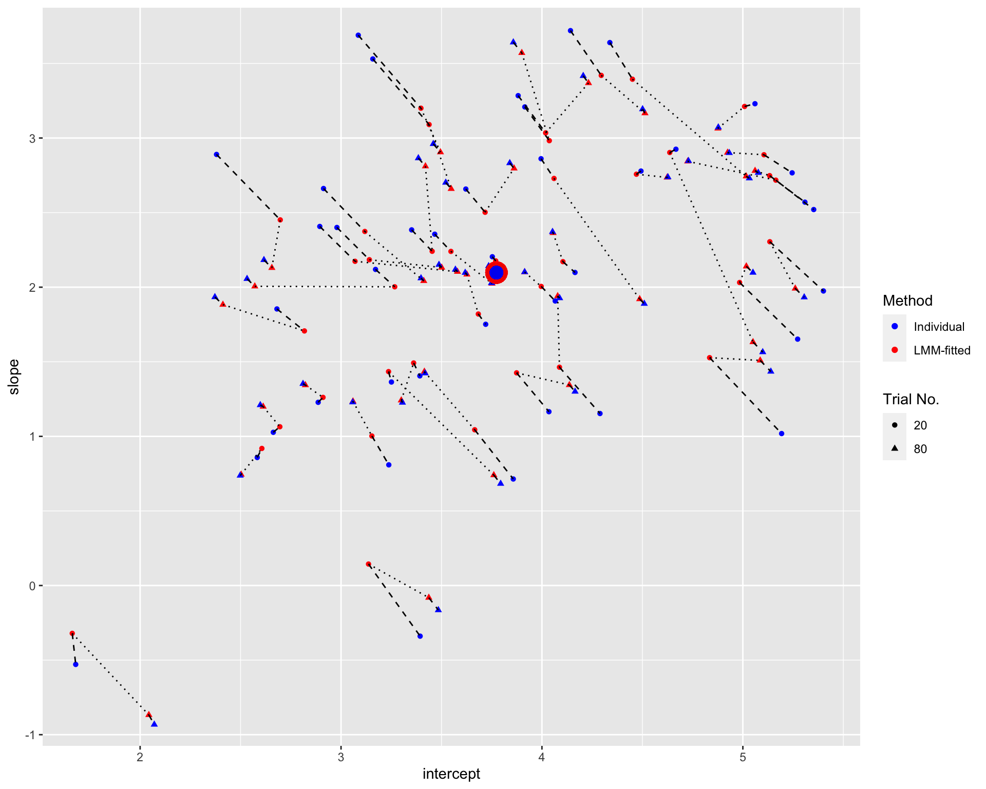 Note: The blue points denote the individual estimates while the red points denote the estimates from linear mixed-effects models. The rounds and triangles denote the estimates with small and large number of trials, respectively. The dashed line connects estimates from different Methods for the same participant and the same number of trials. The dotted line connects the LMM-fitted estimates for the same participant but different numbers of trials. The large points are the population estimates (across all participants).
The figure suggests that the shrinkage is greater for fewer trials, especially for participants who are further away from the population estimates.
5 With varied numbers of trials
After inspecting the shrinkage in separate data sets, the extend of shrinkage is examined in one data set with varied trial numbers for each participant (but the same number of trials in each condition). Specifically, the participant has 10, 20, 30, 40, 50, 60, 70, or 80 trials.
5.1 Simulating data
Simulate the data set:
df_diffN_full <-
  add_random(subj=N_subj) %>%
  add_random(trial=80) %>% # maximal number of trials per participant
  # remove "redundant" trials
  mutate(subjnum = as.integer(substr(subj, 2, 3)),
         trialnum = as.integer(substr(trial, 2, 3)),
         cap = floor((subjnum-1)/5)*10+10) %>%
  filter(trialnum<=cap) %>%
  add_within(IV = c("a1", "a2")) %>%
  add_contrast("IV", "treatment", colnames = "IV_code") %>%
  add_ranef("subj", rand_int = sd_int, rand_slp = sd_slp, .cors=cor_subj) %>%
  add_ranef(sigma = sgm) %>%
  mutate(DV = (fix_int + rand_int) +          # intercept
           (fix_slp + rand_slp) * IV_code +   # slope
           sigma)                        # sigma

df_diffN <- df_diffN_full %>%
  select(Subj=subj, IV, IV_code, Trial=trial, DV)

str(df_diffN)
## tibble [3,600 × 5] (S3: tbl_df/tbl/data.frame)
## $ Subj : chr [1:3600] "s01" "s01" "s01" "s01" ...
## $ IV : Factor w/ 2 levels "a1","a2": 1 2 1 2 1 2 1 2 1 2 ...
## ..- attr(*, "contrasts")= num [1:2, 1] 0 1
## .. ..- attr(*, "dimnames")=List of 2
## .. .. ..$ : chr [1:2] "a1" "a2"
## .. .. ..$ : chr ".a2-a1"
## $ IV_code: num [1:3600] 0 1 0 1 0 1 0 1 0 1 ...
## $ Trial : chr [1:3600] "t01" "t01" "t02" "t02" ...
## $ DV : num [1:3600] 3.31 3 3.71 5.39 3.66 ...The numbers of trials in each condition are:
trialN_diff <- df_diffN %>%
  group_by(Subj, IV) %>%
  summarize(N = n(), .groups = "drop") %>%
  pivot_wider(names_from = IV, values_from = N)

trialN_diff
5.2 Individual estimates
We first estimate the intercepts and slopes for each participant separately (as researchers usually do when employing ANOVAs):
eff_diffN <- df_diffN %>%
  group_by(Subj, IV) %>%
  summarize(avgDV = mean(DV), .groups = "drop") %>%
  pivot_wider(names_from = IV, values_from = avgDV) %>%
  transmute(Subj,
            indi_int = a1,
            indi_slp = a2-a1)

head(eff_diffN)
5.3 LMM-fitted means
Then we estimate the intercepts and slopes for each participant with linear mixed-effects models:
lmm_diffN <- lmer(DV ~ IV + (IV | Subj),
                  data = df_diffN)
summary(lmm_diffN)
## Linear mixed model fit by REML ['lmerMod']
## Formula: DV ~ IV + (IV | Subj)
## Data: df_diffN
##
## REML criterion at convergence: 10570
##
## Scaled residuals:
## Min 1Q Median 3Q Max
## -3.388 -0.670 0.007 0.670 3.333
##
## Random effects:
## Groups Name Variance Std.Dev. Corr
## Subj (Intercept) 1.32 1.15
## IV.a2-a1 1.16 1.08 0.49
## Residual 1.01 1.01
## Number of obs: 3600, groups: Subj, 40
##
## Fixed effects:
## Estimate Std. Error t value
## (Intercept) 3.857 0.184 21.0
## IV.a2-a1 2.043 0.175 11.7
##
## Correlation of Fixed Effects:
## (Intr)
## IV.a2-a1 0.445Extract the intercepts and slopes for each participant:
eff_diffN <- ranef(lmm_diffN) %>%
  as.data.frame() %>%
  transmute(Subj = grp,
            effect = if_else(term=="(Intercept)", "lmm_int", "lmm_slp"),
            condval) %>%
  pivot_wider(names_from = effect, values_from = condval) %>%
  mutate(lmm_int = lmm_int + fixef(lmm_diffN)[1],
         lmm_slp = lmm_slp + fixef(lmm_diffN)[2]) %>%
  inner_join(eff_diffN, by="Subj")

eff_diffN
5.4 Shrinkage
Put all estimates in one data frame:
eff_diffN_long <- eff_diffN %>%
  pivot_longer(contains("_"), names_to = c("Method", "effect"), names_sep="_") %>%
  mutate(effect = if_else(effect=="int", "intercept", "slope"),
         Method = as_factor(Method),
         Method = fct_rev(Method))

str(eff_diffN_long)
## tibble [160 × 4] (S3: tbl_df/tbl/data.frame)
## $ Subj : chr [1:160] "s01" "s01" "s01" "s01" ...
## $ Method: Factor w/ 2 levels "indi","lmm": 2 2 1 1 2 2 1 1 2 2 ...
## $ effect: chr [1:160] "intercept" "slope" "intercept" "slope" ...
## $ value : num [1:160] 2.83 1.42 2.77 1.46 4.68 ...Visualize the shrinkage:
plot_diffN <- eff_diffN_long %>%
  pivot_wider(names_from = effect, values_from = value) %>%
  left_join(trialN_diff, by="Subj") %>%
  mutate(rowname = if_else(Method=="lmm", paste(Subj, a1, sep="_"), ""),
         Method = fct_recode(Method,
                             `LMM-fitted`="lmm",
                             Individual="indi")) %>%
  left_join(eff_diffN %>%
              transmute(Subj,
                        h = ((lmm_int < indi_int)-0.2)*1.5,
                        v = ((lmm_slp < indi_slp)-0.2)*1.5),
            by = "Subj") %>%
  ggplot(aes(intercept, slope)) +
  geom_point(aes(color=Method)) +
  geom_text(aes(label=rowname, hjust=h, vjust=v), size=3) +
  scale_color_manual(values=c("blue", "red")) +
  geom_line(aes(group=Subj), linetype="dashed") +
  geom_point(aes(x = fixef(lmm_diffN)[1],
                 y = fixef(lmm_diffN)[2]),
             size = 7, colour = 'red', alpha = 0.05) +
  geom_point(aes(
    x = mean(eff_diffN$indi_int),
    y = mean(eff_diffN$indi_slp)),
    size = 4, colour = 'blue', alpha = 0.05)

plot_diffN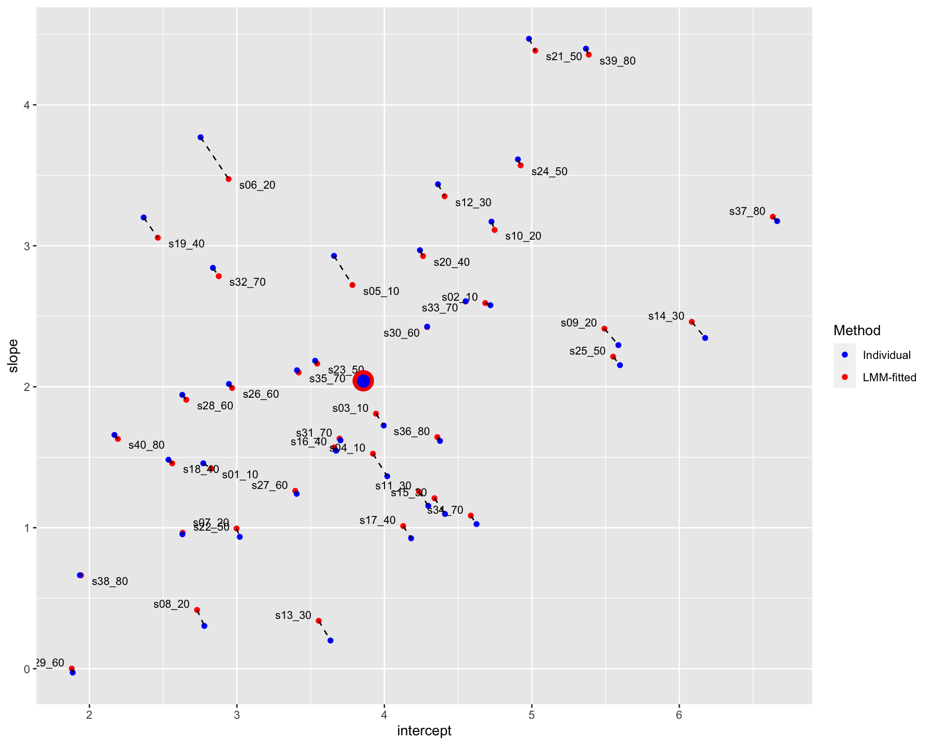 Note: The blue points denote the individual estimates while the red points denote the estimates from linear mixed-effects models. The dashed line connects different estimates for the same participant; the distance between estimates could be understood as the extent of shrinkage. The large points are the population estimates (across all participants). The texts in the figure display the participant code and the number of trials in each condition. For instance, “s06_20” denotes that there is 20 trials in each condition for participant 06.
Similar to the results estimated with separated linear-mixed models, the shrinkage is greater for fewer trials.
6 Take home message
The extent of shrinkage is greater for conditions/participants with fewer trial numbers, especially for participants whose estimates are further away from the population estimates.