(This post was last updated on 2021-04-21.)
Last year, I wrote some codes to simulate data for learning linear mixed models (hierarchical models). It indeed helps me a lot. Recently, I learned a more efficient and decent method of simulating data from this awesome book, and, therefore, summarized it here.
1 Population parameters
In a hypothetical experiment, each of 30 participants viewed all 30 stimuli in different conditions, during which the EEG signals (i.e., the dependent variable) were recorded. The stimuli were presented in different orientations (upright vs. inverted) and with different spatial frequency information (low, medium vs. high).
library(tidyverse)
set.seed(2020)

N_subj <- 30
N_item <- 30

IV1 <- c("upright", "inverted")    # orientation
IV2 <- c("low", "medium", "high")  # spatial frequency
The corresponding parameters of fixed and random effects were assumed as following:
# define the population (fixed effects) parameters
alpha <- -4        # the grand mean
beta_ori <- -2     # orientation: inverted - upright
beta_ml <- -1      # spatial frequency: medium - low
beta_hm <- -.5     # spatial frequency: high - medium
beta_ori_ml <- 1   # interaction between orientation and (medium-low)
beta_ori_hm <- .5  # interaction between orientation and (high-medium)
fixed_true <- c(alpha, beta_ori, beta_ml,
                beta_hm, beta_ori_ml, beta_ori_hm)

# the sigma (residuals)
sigma <- 2

# by-subject random effects
alpha_u_sd <- 2        # sd of the by-subject random intercepts of orientation
beta_ori_u_sd <- .5    # sd of the by-subject random slopes of orientation
beta_ml_u_sd <- .5     # sd of the by-subject random slopes of medium - low
beta_hm_u_sd <- .5     # sd of the by-subject random slopes of high - medium
beta_ori_ml_u_sd <- .5 # sd of the by-subject random slopes of interaction between orientation and (medium-low)
beta_ori_hm_u_sd <- .5 # sd of the by-subject random slopes of interaction between orientation and (high-medium)
u_sd_true <- c(alpha_u_sd, beta_ori_u_sd, beta_ml_u_sd,
               beta_hm_u_sd, beta_ori_ml_u_sd, beta_ori_hm_u_sd)
rho_u <- 0.4           # correlations between the by-subject random effects

# by-item random effects
alpha_w_sd <- 1        # sd of the by-item random intercepts of orientation
beta_ori_w_sd <- .3    # sd of the by-item random slopes of orientation
beta_ml_w_sd <- .3     # sd of the by-item random slopes of medium - low
beta_hm_w_sd <- .3     # sd of the by-item random slopes of high - medium
beta_ori_ml_w_sd <- .3 # sd of the by-item random slopes of interaction between orientation and (medium-low)
beta_ori_hm_w_sd <- .3 # sd of the by-item random slopes of interaction between orientation and (high-medium)
w_sd_true <- c(alpha_w_sd, beta_ori_w_sd, beta_ml_w_sd,
               beta_hm_w_sd, beta_ori_ml_w_sd, beta_ori_hm_w_sd)
rho_w <- 0.3           # correlations between the by-item random effects
1.1 Fixed effects
Create a dataframe to store the experiment conditions:
nlevel_ori <- length(IV1)
nlevel_sf <- length(IV2)
N_cond <- nlevel_ori * nlevel_sf
N_trial <- N_cond * N_subj * N_item

# Create a experiment condition data frame
df_cond <- tibble(
  subject = rep(rep(1:N_subj, each = N_item), each = N_cond),
  stimulus = rep(rep(1:N_item, times = N_subj), each = N_cond),
  Orientation = as_factor(rep(rep(IV1, each = nlevel_sf), times = N_subj * N_item)),
  SF = as_factor(rep(IV2, times = N_subj * N_item * nlevel_ori))
)
# set back difference coding for the independent variables
contrasts(df_cond$Orientation) <- MASS::contr.sdif(nlevel_ori)
contrasts(df_cond$SF) <- MASS::contr.sdif(nlevel_sf)

head(df_cond)
## # A tibble: 6 x 4
## subject stimulus Orientation SF
## <int> <int> <fct> <fct>
## 1 1 1 upright low
## 2 1 1 upright medium
## 3 1 1 upright high
## 4 1 1 inverted low
## 5 1 1 inverted medium
## 6 1 1 inverted highSimulating the fixed effects based on the pre-defined parameters:
# Create the design matrix (including the interaction)
df_simu_design <- model.matrix( ~ 1 + Orientation * SF, df_cond)

# Simulating the fixed effects
dv_fixed <- df_simu_design %*% fixed_true

head(dv_fixed, 10)
## [,1]
## 1 -1.750000
## 2 -3.250000
## 3 -4.000000
## 4 -4.583333
## 5 -5.083333
## 6 -5.333333
## 7 -1.750000
## 8 -3.250000
## 9 -4.000000
## 10 -4.5833331.2 Random effects of subjects
Simulating the random effects of subjects. The codes used here are mainly from this book.
# random effects for subject
N_u_sd <- length(u_sd_true)

# correlation matrix
u_corr <- (1- diag(N_u_sd)) * rho_u + diag(N_u_sd)
# Cholesky factor
L_u <- chol(u_corr)
# # We  can verify that we recover rho_u with:
# t(L_u) %*% L_u

# simulate random effects for subjects
# uncorrelated z values from the standard normal distribution for all random effects
z_u <- replicate(N_u_sd, rnorm(N_subj, 0, 1))
# Variance matrix
u_var <- diag(N_u_sd) * u_sd_true

# random effects of subjects
u <- u_var %*% t(L_u) %*% t(z_u)
random_u <- t(u)[df_cond$subject, ]

# random effects of subjects for each trial
dv_u <- rowSums(df_simu_design * random_u)

head(dv_u, 10)
## 1 2 3 4 5 6 7 8 9 10
## 0.4779032 1.3330333 0.8963092 0.2875238 1.0471456 0.4817504 0.4779032 1.3330333 0.8963092 0.28752381.3 Random effects for items
# random effects for item
N_w_sd <- length(w_sd_true)

# correlation matrix
w_corr <- (1- diag(N_w_sd)) * rho_w + diag(N_w_sd)
# Cholesky factor
L_w <- chol(w_corr)
# # We verify that we recover rho_w,
# t(L_w) %*% L_w

# simulate random effects for subjects
# uncorrelated z values from the standard normal distribution for all random effects
z_w <- replicate(N_w_sd, rnorm(N_subj, 0, 1))
# Variance matrix
w_var <- diag(N_w_sd) * w_sd_true

# random effects of items
w <- w_var %*% t(L_w) %*% t(z_w)
random_w <- t(w)[df_cond$stimulus, ]

# random effects of items for each trial
dv_w <- rowSums(df_simu_design * random_w)

head(dv_w, 10)
## 1 2 3 4 5 6 7 8 9 10
## -0.11608704 -0.17042700 -0.74480601 -0.03791199 0.06551072 -0.65235263 0.91065516 1.00563328 0.62334341 0.877647891.4 Generate the dependent variables
Combine the fixed, random effects and the sigma:
# combine fixed, random effects and the sigma (residuals)
df_simu <- df_cond %>%
  mutate(erp = dv_fixed + dv_u + dv_w + rnorm(n(), 0, sigma))

head(df_simu, 10)
## # A tibble: 10 x 5
## subject stimulus Orientation SF erp[,1]
## <int> <int> <fct> <fct> <dbl>
## 1 1 1 upright low 0.824
## 2 1 1 upright medium -7.20
## 3 1 1 upright high -6.30
## 4 1 1 inverted low -4.58
## 5 1 1 inverted medium -2.61
## 6 1 1 inverted high -5.64
## 7 1 2 upright low 4.84
## 8 1 2 upright medium -1.21
## 9 1 2 upright high -1.46
## 10 1 2 inverted low -7.262 Fitting the model
Bayesian hierarchical modeling was used to estimate the parameters.
library(brms)
library(bayesplot)
# The "full" model
fit_simu <- brm(erp ~ Orientation * SF +
(Orientation * SF | subject) +
(Orientation * SF | stimulus),
data = df_simu,
prior = c(
prior(normal(-4, 5), class = Intercept),
prior(normal( 0, 5), class = b),
prior(normal( 5, 5), class = sigma),
prior(normal( 0, 2), class = sd),
prior(lkj(2), class = cor)
),
cores = 10,
chains = 10,
warmup = 2000,
iter = 4000,
file = "2020-09-12-brm_simulation")
summary(fit_simu)## Family: gaussian
## Links: mu = identity; sigma = identity
## Formula: erp ~ Orientation * SF + (Orientation * SF | subject) + (Orientation * SF | stimulus)
## Data: df_simu (Number of observations: 5400)
## Samples: 10 chains, each with iter = 4000; warmup = 2000; thin = 1;
## total post-warmup samples = 20000
##
## Group-Level Effects:
## ~stimulus (Number of levels: 30)
## Estimate Est.Error l-95% CI u-95% CI Rhat Bulk_ESS Tail_ESS
## sd(Intercept) 1.09 0.15 0.83 1.43 1.00 2918 5428
## sd(Orientation2M1) 0.39 0.09 0.23 0.59 1.00 8074 10600
## sd(SF2M1) 0.35 0.10 0.17 0.55 1.00 7582 8468
## sd(SF3M2) 0.19 0.11 0.01 0.41 1.00 4711 5950
## sd(Orientation2M1:SF2M1) 0.17 0.13 0.01 0.49 1.00 9294 9022
## sd(Orientation2M1:SF3M2) 0.23 0.15 0.01 0.57 1.00 8299 9105
## cor(Intercept,Orientation2M1) 0.12 0.20 -0.28 0.49 1.00 12704 14559
## cor(Intercept,SF2M1) 0.32 0.20 -0.11 0.68 1.00 16151 14805
## cor(Orientation2M1,SF2M1) 0.20 0.24 -0.30 0.65 1.00 11950 14099
## cor(Intercept,SF3M2) 0.02 0.28 -0.53 0.55 1.00 22699 14173
## cor(Orientation2M1,SF3M2) -0.07 0.29 -0.62 0.51 1.00 16396 14276
## cor(SF2M1,SF3M2) 0.08 0.30 -0.50 0.64 1.00 15530 15394
## cor(Intercept,Orientation2M1:SF2M1) -0.03 0.32 -0.64 0.59 1.00 28044 14044
## cor(Orientation2M1,Orientation2M1:SF2M1) 0.03 0.33 -0.61 0.63 1.00 25867 15222
## cor(SF2M1,Orientation2M1:SF2M1) 0.06 0.32 -0.58 0.66 1.00 22419 15812
## cor(SF3M2,Orientation2M1:SF2M1) 0.04 0.33 -0.60 0.65 1.00 17031 15859
## cor(Intercept,Orientation2M1:SF3M2) 0.25 0.31 -0.43 0.76 1.00 20346 14389
## cor(Orientation2M1,Orientation2M1:SF3M2) 0.03 0.31 -0.56 0.62 1.00 23547 15375
## cor(SF2M1,Orientation2M1:SF3M2) 0.09 0.31 -0.53 0.66 1.00 20585 15709
## cor(SF3M2,Orientation2M1:SF3M2) 0.11 0.33 -0.54 0.70 1.00 16056 16285
## cor(Orientation2M1:SF2M1,Orientation2M1:SF3M2) -0.11 0.34 -0.72 0.57 1.00 12812 15768
##
## ~subject (Number of levels: 30)
## Estimate Est.Error l-95% CI u-95% CI Rhat Bulk_ESS Tail_ESS
## sd(Intercept) 2.65 0.34 2.08 3.40 1.00 3028 5322
## sd(Orientation2M1) 0.31 0.09 0.13 0.50 1.00 6211 4849
## sd(SF2M1) 0.69 0.13 0.48 0.97 1.00 8084 11804
## sd(SF3M2) 0.50 0.11 0.30 0.73 1.00 8331 11983
## sd(Orientation2M1:SF2M1) 0.79 0.20 0.42 1.21 1.00 8567 9960
## sd(Orientation2M1:SF3M2) 0.53 0.19 0.15 0.92 1.00 6839 4387
## cor(Intercept,Orientation2M1) -0.03 0.21 -0.44 0.38 1.00 15161 14331
## cor(Intercept,SF2M1) 0.09 0.18 -0.27 0.43 1.00 9590 12711
## cor(Orientation2M1,SF2M1) -0.01 0.23 -0.45 0.44 1.00 3789 7097
## cor(Intercept,SF3M2) 0.17 0.19 -0.21 0.52 1.00 13441 13638
## cor(Orientation2M1,SF3M2) 0.29 0.24 -0.21 0.71 1.00 6605 10651
## cor(SF2M1,SF3M2) -0.03 0.22 -0.44 0.40 1.00 9896 13671
## cor(Intercept,Orientation2M1:SF2M1) 0.17 0.20 -0.24 0.55 1.00 14735 14682
## cor(Orientation2M1,Orientation2M1:SF2M1) 0.18 0.25 -0.32 0.65 1.00 7144 11502
## cor(SF2M1,Orientation2M1:SF2M1) 0.24 0.22 -0.21 0.64 1.00 13221 14167
## cor(SF3M2,Orientation2M1:SF2M1) -0.07 0.24 -0.51 0.40 1.00 12067 14652
## cor(Intercept,Orientation2M1:SF3M2) 0.48 0.22 -0.00 0.82 1.00 15444 11363
## cor(Orientation2M1,Orientation2M1:SF3M2) 0.04 0.27 -0.48 0.55 1.00 15815 15037
## cor(SF2M1,Orientation2M1:SF3M2) 0.07 0.26 -0.44 0.56 1.00 18386 15649
## cor(SF3M2,Orientation2M1:SF3M2) 0.17 0.26 -0.37 0.64 1.00 16331 15535
## cor(Orientation2M1:SF2M1,Orientation2M1:SF3M2) 0.28 0.26 -0.26 0.74 1.00 14719 13953
##
## Population-Level Effects:
## Estimate Est.Error l-95% CI u-95% CI Rhat Bulk_ESS Tail_ESS
## Intercept -3.74 0.54 -4.81 -2.67 1.01 1063 1904
## Orientation2M1 -1.91 0.11 -2.13 -1.70 1.00 8954 12363
## SF2M1 -0.85 0.16 -1.17 -0.55 1.00 6702 10557
## SF3M2 -0.63 0.12 -0.86 -0.39 1.00 9816 12962
## Orientation2M1:SF2M1 1.12 0.20 0.72 1.52 1.00 11505 14224
## Orientation2M1:SF3M2 0.50 0.17 0.16 0.85 1.00 8036 12473
##
## Family Specific Parameters:
## Estimate Est.Error l-95% CI u-95% CI Rhat Bulk_ESS Tail_ESS
## sigma 1.99 0.02 1.96 2.03 1.00 25648 15240
##
## Samples were drawn using sampling(NUTS). For each parameter, Bulk_ESS
## and Tail_ESS are effective sample size measures, and Rhat is the potential
## scale reduction factor on split chains (at convergence, Rhat = 1).2.1 Compare the estimated and population parameters
Comparisons between the population (True) and estimated parameters of fixed effects: (Note: the True values are the population parameters used to simulate the data.)
as.data.frame(fit_simu) %>%
  select(starts_with("b_")) %>%
  mcmc_recover_hist(true = fixed_true)
## `stat_bin()` using `bins = 30`. Pick better value with `binwidth`.
Comparisons between the population (True) and estimated parameters of by-subject random effects:
as.data.frame(fit_simu) %>%
  select(starts_with("sd_subject")) %>%
  mcmc_recover_hist(true = u_sd_true)
## `stat_bin()` using `bins = 30`. Pick better value with `binwidth`.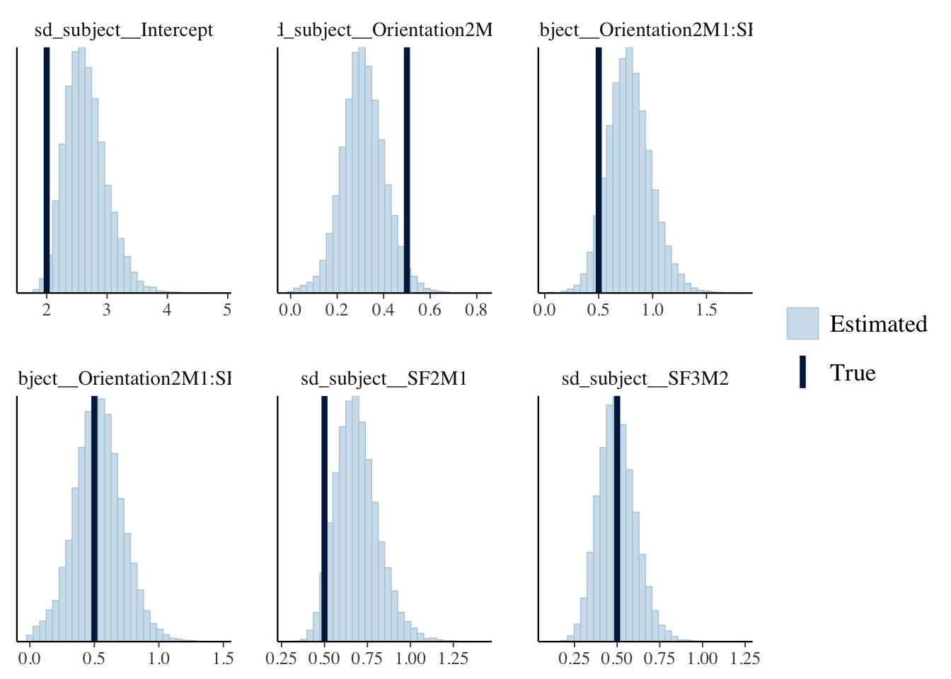
Comparisons between the population (True) and estimated parameters of by-item random effects:
as.data.frame(fit_simu) %>%
  select(starts_with("sd_stimulus")) %>%
  mcmc_recover_hist(true = w_sd_true)
## `stat_bin()` using `bins = 30`. Pick better value with `binwidth`.
3 Update: simulate data with a function
The above codes are wrapped into a function, which can be used as follows:
# source the function
devtools::source_gist("https://gist.github.com/HaiyangJin/097e33a79597ec73bcbf419c428086c1")
# simulate data
simu_func <- simudata_lmm2()
To get the simulated data:
# obtain the simulated data
df_simu_gist23 <- simu_func$simudata %>%
   mutate(Orientation = as.character(Orientation),
          SF = as.character(SF))
str(df_simu_gist23)
## tibble[,5] [5,400 × 5] (S3: tbl_df/tbl/data.frame)
## $ subject : int [1:5400] 1 1 1 1 1 1 1 1 1 1 ...
## $ stimulus : int [1:5400] 1 1 1 1 1 1 2 2 2 2 ...
## $ Orientation: chr [1:5400] "upright" "upright" "upright" "inverted" ...
## $ SF : chr [1:5400] "low" "medium" "high" "low" ...
## $ erp : Named num [1:5400] 1.181 0.416 -1.418 -0.274 -1.283 ...
## ..- attr(*, "names")= chr [1:5400] "1" "2" "3" "4" ...Note that the design for the simulated data is 2 \(\times\) 3, but you may only analyze subset of the data (e.g., 2 \(\times\) 2 design).
df_simu_gist22 <- df_simu_gist23 %>%
  filter(SF != "medium")
str(df_simu_gist22)
## tibble[,5] [3,600 × 5] (S3: tbl_df/tbl/data.frame)
## $ subject : int [1:3600] 1 1 1 1 1 1 1 1 1 1 ...
## $ stimulus : int [1:3600] 1 1 1 1 2 2 2 2 3 3 ...
## $ Orientation: chr [1:3600] "upright" "upright" "inverted" "inverted" ...
## $ SF : chr [1:3600] "low" "high" "low" "high" ...
## $ erp : Named num [1:3600] 1.181 -1.418 -0.274 -4.203 -4.221 ...
## ..- attr(*, "names")= chr [1:3600] "1" "3" "4" "6" ...Also, you may obtain the “true” values used for simulating the data:
# true values used to simulate the data
simu_func$population
## upr_low upr_med upr_hig inv_low inv_med inv_hig
## -1.750000 -3.250000 -4.000000 -4.583333 -5.083333 -5.333333With “true” values, you may calculate the differences to check whether they match some of the parameters of the fitted model.
Enjoy!